Replica exchange nested sampling

To get the most out of this section, you should already be familiar with the basics of nested sampling (NS). If not, feel free to check out this gentle introduction first.

The shortcomings of MCMC

We’ve seen that to generate independent samples from the constrained regions at each NS iteration, Markov-chain Monte Carlo (MCMC) random walks are typically employed. While MCMC is essentially the only viable method for sampling in high-dimensional systems, it also comes with serious limitations.

To illustrate this, consider the bimodal energy surface shown in the visualization below. This surface has been deliberately constructed with a broad, shallow high-energy basin and a significantly narrower, deeper global minimum. Such a structure poses a challenge for NS, which operates top-down by evolving walkers from higher to lower energy regions. For the process to succeed, MCMC chains must "find the entry" to the global minimum at the right moment.

Click through the visualization to see how this may fail in practice.

While exploring the visualization, pay attention to the following:

• Entry closing: at iteration 9 the entry to the global minimum mode is about to close.
• Barrier formation: From iteration 10 onward, an infinitely high barrier forms between the metastable and global minimum basins.

Once this barrier has formed, it becomes exceedingly unlikely for MCMC to re-enter the global minimum. A successful transition would require a large, well-directed step—something increasingly improbable as the barrier widens.

While the example surface may seem overly idealized, similar situations are common in materials simulations. First-order phase transitions—such as the shift from a liquid to a crystalline phase—often involve dramatic reductions in accessible phase space. In this analogy, the liquid phase corresponds to the broad, high-energy basin, while the crystalline phase represents the narrow, low-energy well.

RENS – Cooperative NS Simulations

What if we could run several NS simulations in parallel and allow them to cooperate?

Replica exchange (RE) provides a statistical framework for exchanging samples between different distributions, while rigorously preserving the statistics of each one. Since the walkers at NS iteration are drawn from the likelihood-constrained prior,

RE gives us a principled way to exchange configurations between different NS runs. A more formal description can be found in this work.

To introduce the idea of replica-exchange nested sampling (RENS), let’s return to the bimodal energy surface. While not the most sophisticated use case, it’s illustrative. Suppose we run two NS simulations in parallel. The standard NS procedure continues in each, but we now periodically perform RE swap moves. The swap rule at iteration is simple:

This mechanism is best understood by walking through a concrete example. The visualization below shows both simulations (we call them replica and now), with their walkers represented as small red circles. In the panel of simulation , we indicate the swap candidate as a full yellow circle and the potential swap partner from simulation as empty yellow circle and for simulation the other way around. Furthermore, we indicate whether a swap attempt was accepted or rejected by a ACC/REJ tag respectively.

Clicking through the simulation you should see the following:

• In simulation , the global minimum basin becomes disconnected at iteration 14.
• From then on, the global minimum is no longer sampled—an independent NS run would be stuck.
• Simulation successfully enters the global minimum basin at iteration 11.
• At iteration 19, a walker from residing in the global minimum is swapped into —repopulating the previously lost region.
• Initially, most swaps are accepted, but the acceptance rate gradually decreases.

Introducing a new toy model

The previous example used a simple 2D bimodal energy surface. Let’s now introduce a toy model that’s a bit closer to real-world materials simulations. We consider a periodic chain of particles interacting via the pair potential shown below:

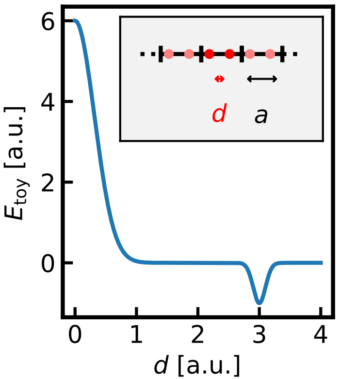
We represent the system as two particles in a periodically repeated box. Due to translational invariance, we can fix one particle at zero and move only the second one. This gives us two degrees of freedom:

• The lattice parameter (box size),
• The position of the second particle (interparticle distance).

The visualization below shows the 2D configuration space, along with the unit cell and its two particles. You can interact with and and enable periodic boundary conditions (apply PBC) to observe how the particle gets mapped back into the cell. You’ll see that, due to periodicity, it's sufficient to only consider the upper triangular part of configuration space (irred. only). Finally, an external pressure can be applied to the system, significantly reshaping the energy landscape.

Pressure RENS

This setup lets us apply RENS in a much more compelling scenario: simulations with different energy landscapes. Recall that the acceptance probability of RE swaps depends critically on the overlap between the involved distributions. If the distributions differ too much, swaps will rarely be accepted. This is where materials science offers a natural use case: an external pressure introduces a continuous deformation of the energy (more precisely, enthalpy) landscape. Because we often want to compute NS partition functions across a range of pressures anyway, this structure is a perfect match for RENS. Below you can explore a simple example using two replicas—one at lower pressure (left), one at higher pressure (right).

Observe how pressure subtly reshapes the likelihood-constrained distributions. It’s precisely this controlled diversity across simulations that gives RENS its true strength. Unlike the simplified two-replica examples shown here, RENS is typically applied with many replicas—often around 10—each exploring slightly different conditions. Think of it like a team of skilled football players, each with their own specialty, working together to cover the entire field more effectively than any individual could alone.

Predicting the silicon phase diagram with RENS

While the toy system serves as a useful illustration of the core idea behind RENS, I now want to demonstrate a real-world application. We used RENS to predict the silicon phase diagram using a neural-network force field (NNFF) trained on density functional theory (DFT) data.

Constructing a 2D configuration space map

We consider a unit cell containing silicon atoms. The corresponding configuration space is high-dimensional—roughly dimensions. To gain some insight into the processes taking place in this space, we apply a dimensionality reduction technique that leverages our training data.

For each configuration in the training set, we compute two structural order parameters and evaluate their enthalpies using . We then interpolate between these configurations in the 2D order parameter space. The interactive visualization below illustrates this interpolation using a triangulation-based method to generate a continuous surface. You can vary the pressure between 2 and 16 GPa.

You can observe the following features:

• High-energy configurations (e.g., liquid or gas-like) are located in the upper right.
• Low-energy crystalline phases are found at the bottom.
• Two major crystalline regions can be distinguished:
  • Bottom left: high-density phases such as simple hexagonal.
  • Bottom right: low-density phases such as cubic diamond.
• Note how pressure alters the relative enthalpies of these phases: higher pressures stabilize high-density phases and destabilize low-density ones.

Independent NS

Using this 2D configuration map, we now examine a set of independent NS simulations performed with walkers and MCMC steps. These simulations required approximately energy evaluations in total.

The following visualization shows simulations at four intermediate pressures between 8 and 14 GPa—a region that turns out to be particularly challenging due to the complex interplay between several crystalline phases. In each frame:

• Walker configurations are shown as red circles.
• Acquired NS samples appear as empty grey circles.
• The highest-energy walker (i.e., the current NS sample) is highlighted in light-blue.

Since the simulations ran for ~150,000 iterations, we do not show every frame to save space. Instead, we display samples from every other iteration and update walker sets only at longer intervals. (Note: some visual glitches remain in the current version. I will try to fix them soon)

While stepping through the animation, observe the following:

• Walker clouds typically begin in the high-energy region (top right) and move diagonally toward the bottom left.
• Around frame 55, the walker cloud splits into two—this corresponds to a liquid-solid phase transition.
• Toward the end, the walkers condense around a single point, corresponding to a minimum on the enthalpy surface.
• Interestingly, each simulation settles into a different final state, suggesting four stable phases between 8 and 14 GPa.

However, as we will see next, this variability of outcomes is an artifact of failing independent NS simulations rather than physical reality.

RENS

Let’s now re-examine the same pressure range using RENS, with the same parameters: walkers and MCMC steps. Note that the computational cost—measured in energy evaluations—is identical to that of the independent NS runs.

Without further ado, check out the same visualization for pressures 8 to 14 GPa using RENS:

You should notice that the RENS simulations consistently converge toward only two final states:

• For pressures from 8 to 12 GPa, the simulation ends in the low-density phase (bottom right).
• At 14 GPa, it ends in the high-density phase (bottom left).

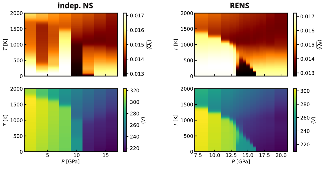
What we observe in configuration space also shows up in thermodynamic observables. The figure below shows the pressure dependence of two expectation values: the volume and a structural order parameter, specifically the mean Steinhardt bond order parameter .

In the independent NS simulations, both observables show strong, unphysical fluctuations between neighboring pressures. The phase transition is also mispredicted to occur around 10 GPa, far below the expected value of ~14 GPa. By contrast, RENS yields a smooth phase diagram for both volume and , with the transition point much closer to the expected value.

If this sparked your interest, feel free to explore our paper, for an in-depth introduction to RENS:

Unglert, N.; Pártay, L. B.; Madsen, G. K. H. Replica Exchange Nested Sampling. J. Chem. Theory Comput. 2025, 21 (15), 7304–7319. https://doi.org/10.1021/acs.jctc.5c00588.